Lately many exciting results with deep learning in radiology have been reported. This is not that much of a surprise, as deep learning is eminently suited for medical image analysis. Deep learning algorithms have been shown to be capable of analyzing many different medical images with high accuracy. Examples are chest X-rays, mammograms, breast MRIs and cardiac MRIs,1–5 but there are many more examples out there.
All these results are very promising, but what is actually inside the black box of deep learning? How do you build a deep neural network?
Deep neural network: the structure
To gain a better understanding of how to build a deep neural network, we need to understand all the elements a neural network contains. A neural network consists of layers, each consisting of nodes. There is an input layer which can be the image, or parts of the image. Then, there are several hidden layers which have the function of extracting image features. Lastly, there is the output layer answering the question the network is supposed to answer.
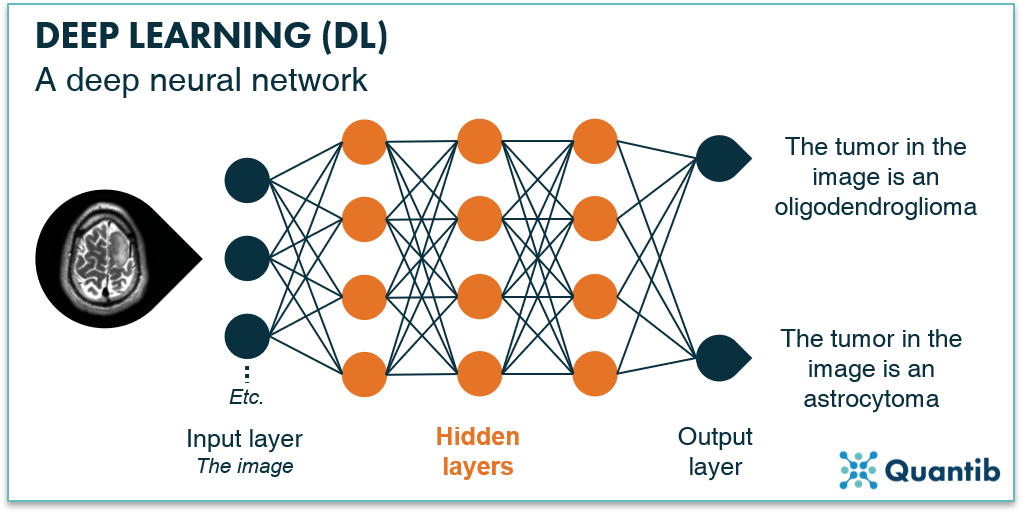
Figure 1: A deep neural network consists of an input layer, multiple hidden layers and an output layer, all consisting of nodes.
A node represents a basic calculation: it takes an input and calculates an output. The input consists of the output from all nodes in the previous layer (hence the connecting lines between nodes in figure 1). Inside the node, the output gets calculated and it is passed on to the next layer. Training your deep neural network is nothing more than figuring out the optimal output for each node, so that when all nodes are combined, the network gives the right response.
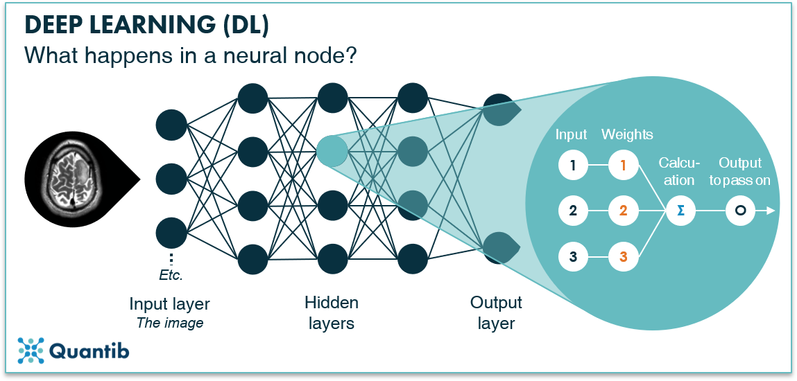
Figure 2: A node in a hidden layer of a deep neural network takes an input, performs a calculation, and passes on an output to nodes in the next layer.
The calculation consists of two parts: 1) a simple multiplication of all the inputs by the related “weight”, and 2) the activation function. In the first part, each input is multiplied with a corresponding weight and the outcomes are summed. The second part, the activation function, is a bit more complex. It allows the network to perform more complex calculations, and thus, solve more advanced problems. After applying these two steps, the output of the node is passed on to multiple nodes in the next layer (to whom it becomes an input). See figure 3 for a visual explanation of the calculation within a neural node. In a traditional neural network, usually the hidden layers are fully connected, meaning each node in the first hidden layer is connected to each node in the second, which is connected to each node in the third hidden layer, etc.
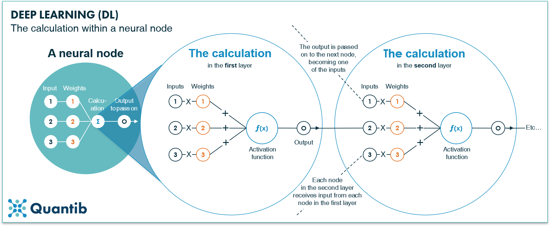
Figure 3: Each neural node in a deep neural network performs a calculation by taking inputs from nodes in the previous layer, multiplying these by weights, and summing all outcomes. The resulting number gets processed by an activation function to allow for more complex calculations. Lastly, the output is passed on to the nodes in the next layer.

Building a neural network in 3 steps
As we saw in the previous section, the weights of a neural network directly influence how input data is transformed and passed on from one node to the next. Hence, in the end, the weights control the value of the output. The process of determining the value of weights that give the correct output is called training. To get a grasp of how many weights we are dealing with, see figure 4.
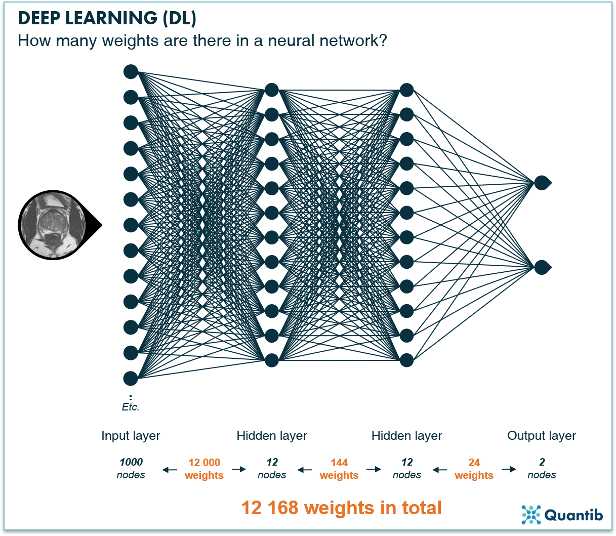
Figure 4: If the input layer (the image) consists of 10x10x10 voxels, you already start with 1000 nodes. Say your neural network contains two hidden layers with each 12 nodes and 2 output nodes, stating whether the input image does or does not contain a tumor. For each connection shown in the figure above, you need a weight, so this very simple network contains 1000 x 12 + 12 x 12 +2*12 = 12 168 weights.
In order to correctly train a deep neural network, example data is needed. This data consists of examples (in the case of deep learning in radiology, these are usually medical images) containing input and the corresponding correct output, i.e. the ground truth. The training procedure is usually performed using 3 independent datasets, each containing different examples: a training set, a validation set, and a test set. The datasets are used in three different steps of the training process.
Step 1: Initial training of the network using the training set
The first step is training of the network, i.e. taking a go at determining the value of each weight. This is done using backpropagation.
To train the network using backpropagation, you start by assigning all weights to random values. Subsequently, every image in the training set is run through the network. The output of the network, which will be completely random at this stage, is then compared to our ground truth. The difference between the output and the ground truth can be expressed as an error. For example, our network is supposed to compute the probability that our image contains a tumor. We insert an image containing a tumor and the network returns “32% chance of a tumor”. Comparing this response with the ground truth, in this case “100% chance of a tumor”, we can estimate an error of 68%, meaning the algorithm is pretty far off.
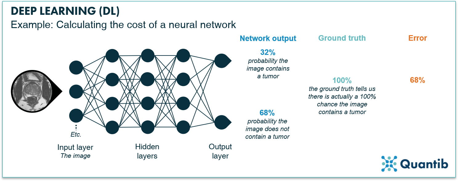 Figure 5: Calculation of error of one image. The image passes through the network generating an output. In this case, the network returns a 32% probability that a tumor is present in the image (and therefore a probability of 68% of the image not containing a tumor). The error is given by the difference between the ground truth, 100% probability of the image containing a tumor, and the output of the network, 32% probability of the image containing a tumor. Thus, the error is 68%.
The error of each example in the training set is then combined to obtain the total error of the network over the training set, which is nothing more than summing up the error for all images in the training set.
For our network to have an optimal performance, we need to minimize this total error. Stage enter backpropagation calculation. This is achieved by adjusting all weights starting at the output layer and working our way back to the input layer. A commonly used method to iteratively adjust the weights, slowly approaching the right values, is called gradient descent. We will discuss this technique in a future blog post!
Step 2: Refining the network using the validation set
The training procedure described above will provide a neural network that has a very small error when applied to the training set. Roughly speaking, we can say that the deeper the network, i.e. the more hidden layers and more nodes it has, the better it is at learning from the training set. What might happen, however, is that the network learns too much from the given examples, or in other words, it overfits. This results in a great performance of the network on the training set, but a poor performance with new data. In other words, the network's performance is not generalizable.
To overcome overfitting, an independent dataset is used to evaluate the network's performance. This is the validation set. This is done during training, so we can check whether the algorithm performs well on the training set, but lousy on the validation set. If this is the case, you have overfitted and you will need to go back to the drawing board to make adjustments. There are several ways to do this. For example, you could:
- Use more data. This is easier said than done, because usually if you had more data at the start, you would have used it already.
- Apply augmentation. If there is not enough original data available, it can be created in an artificial way. Take the original dataset and transform the images such that they are different, but still resemble a credible example. This transformation may be cropping, translating, rotating, resizing, stretching, or randomly deforming them. We will discuss augmentation in a future blog post!
- Apply drop out. This method is applied during training of the network by ignoring random neurons with each iteration during training, i.e. “turning them off”. By doing this, other neurons will pick up the task of the ignored neurons. Hence, instead of the network becoming too dependent on specific weights between specific neurons, the interdependencies distribute themselves over the whole network.6
- Apply regularization to the weights. By introducing other conditions or extra controls on the weights, or actually the total of all weights, you can steer the network away from overfitting.
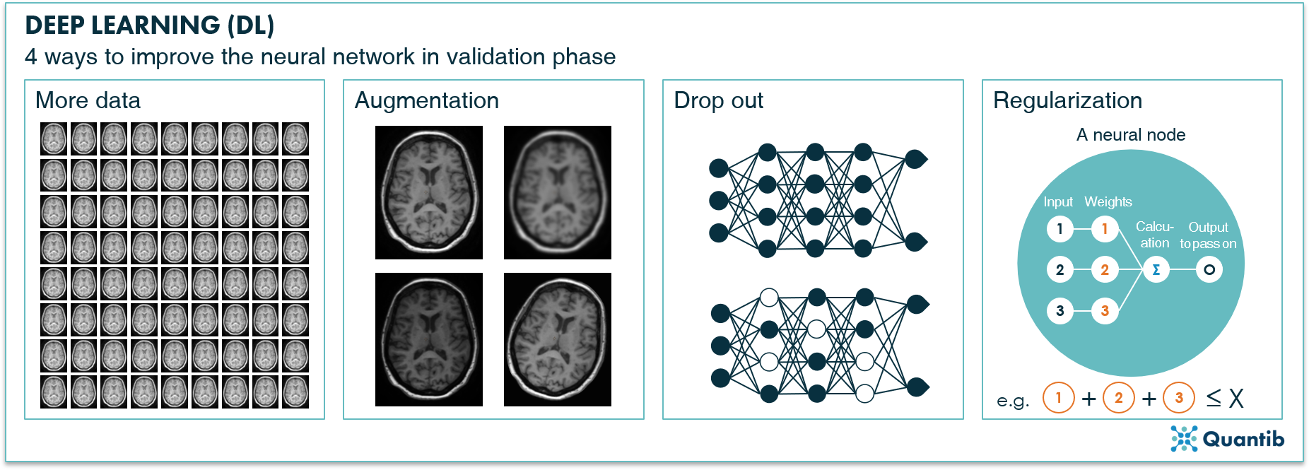 Figure 6: There are several ways to improve the algorithm in case of overfitting: adding more data to the training set, performing augmentation, applying drop out, or regularization.
Step 3: Using the test set
The very last step, testing, uses a set of data that has been kept apart. This step is very straightforward: the algorithm processes the images in the test set and performance measurements, such as accuracy, recall, or DICE score are calculated. Hence, this is an independent test of how the algorithm performs on data that has not been seen before. After the algorithm performance has been checked using this test set, there is no going back. After all, tweaking the algorithm based on the test results, would make the test set everything but unrelated to the training of the network.
Curious to learn more about artificial intelligence in radiology? Visit our Ultimate Guide to AI in radiology.

Bibliography
- Ridley, E. L. AI outperforms physicians for interpreting chest x-rays. (2019). Available at: https://www.auntminnie.com/index.aspx?sec=sup&sub=xra&pag=dis&ItemID=125040. (Accessed: 12th April 2019)
- Ridley, E. L. AI and radiologists: Better together in screening mammo. (2019). Available at: https://www.auntminnie.com/index.aspx?sec=sup&sub=aic&pag=dis&ItemID=125004 . (Accessed: 12th April 2019)
- McKinney, S.M. et al. International evaluation of an AI system for breast cancer screening. (2020). Available at: https://www.nature.com/articles/s41586-019-1799-6
- Witowski, J. et al. Improving breast cancer diagnostics with artificial intelligence for MRI. (2022). Available at: https://www.medrxiv.org/content/10.1101/2022.02.07.22270518v1
- Forrest, W. Deep learning with MRI mimics cardiac technologists. Available at: https://www.auntminnie.com/index.aspx?sec=road&sub=def&pag=dis&ItemID=123333.
- Cicuttin, A. et al. A programmable System-on-Chip based digital pulse processing for high resolution X-ray spectroscopy. 2016 Int. Conf. Adv. Electr. Electron. Syst. Eng. ICAEES 2016 15, 520–525 (2017).